Fluorescence Model
FluorescenceModel is the main entry point for building
fluorescence models. Given a solar pumping spectrum
and physical parameters, it solves for level populations and synthesises a
spectrum convolved with a line-spread function (LSF). All inputs and outputs
use Å for wavelength and erg s-1 cm-2 Å-1 for flux.
Sections
Solar Irradiance at the comet
The first thing a fluorescence model needs is the solar irradiance spectrum at the comet frame, which is the spectrum that will pump the molecules radiatively.
You can provide any solar spectrum, but it must first be transformed to the comet frame (scaled by the heliocentric distance and Doppler-shifted by the comet velocity)
and have columns named WAVE and FLUX. Alternatively, you can use the defaults shipped with cometspec:
the Kurucz solar model [1] from 2990 to 10,000 Å and the Hall & Anderson spectrum [2] from 2000 to 2990 Å.
Check the Solar irradiance section in Utilities for more options.
from cometspec.helper import open_kurucz_irradiance, open_hall_anderson_irradiance

irradiance_kurucz = open_kurucz_irradiance()
irradiance_hall_anderson = open_hall_anderson_irradiance()
You then can concatenate them to extend it to 2000 Å.
import numpy as np
import pandas as pd

flux_kurucz = irradiance_kurucz['FLUX']
flux_hall_anderson = irradiance_hall_anderson['FLUX']

wave_kurucz = irradiance_kurucz['WAVE']
wave_hall_anderson = irradiance_hall_anderson['WAVE']

wave = np.concatenate([wave_hall_anderson, wave_kurucz])
flux = np.concatenate([flux_hall_anderson, flux_kurucz])

irradiance = pd.DataFrame({'WAVE': wave, 'FLUX': flux})
The wavelength range used to filter the default transition linelists is taken directly
from the minimum and maximum wavelengths of the supplied solar irradiance (pumping)
spectrum, so simply passing a concatenated irradiance that extends down to 2000 Å
is enough to make those lines available.
Remember to correct the wavelengths for the comet’s heliocentric velocity and to
scale the flux by the heliocentric distance.
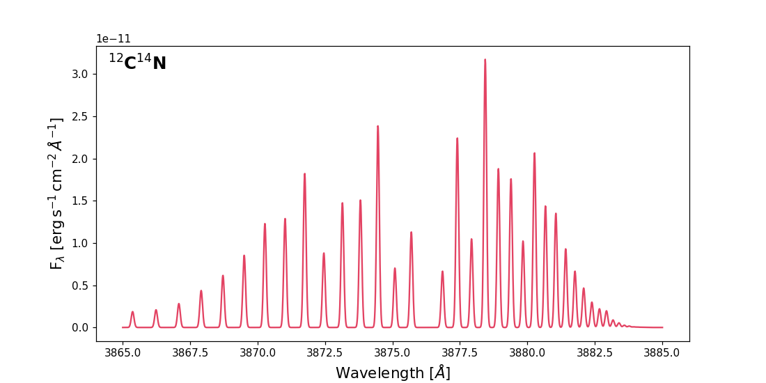
One-isotopologue model
Build a model for 12C14N.
Note
The collisional parameter f_col used throughout these docs is defined as
where the same downward rate \(C_{ul}\) is assumed for every upper-to-lower pair included in the collision scaffold.
from cometspec import FluorescenceModel

model = FluorescenceModel(
   pumping=irradiance,
   isotopologues="12C14N",
   window = (3865, 3885),
   logN=14.0,        # log10 column density [moelcules cm^-2]
   T=100.0,          # Kinetic temperature [K]
   f_col=-1,         # f_col = log10(C_ul / s^-1)
   sigma=0.05,        # Gaussian LSF sigma [Å]
   A_min=1e3,         # Minimum einstein A for lines to include
   lsf_method="Gauss",
   include_rotations=True,  # Whether to include collisions
)
The model automatically loads the Brooke et al. CN line list [3], builds the
radiative rate matrix, solves for the level populations assuming equilibrium, and synthesises the spectrum.
The result is stored in the best_model attribute.
To plot it:
from matplotlib import pyplot as plt

plt.figure(figsize=(10, 5))
plt.text(0.02, 0.97, r"$^{12}$C$^{14}$N", transform=plt.gca().transAxes,
         fontsize=16, fontweight="bold", va="top")
plt.plot(model.model_wave, model.best_model, c='crimson', alpha=0.8)
plt.xlabel(r"Wavelength [$\AA$]", fontsize=14)
plt.ylabel(r"F$_\lambda$ [$\mathrm{erg}\,\mathrm{s}^{-1}\,\mathrm{cm}^{-2}\,\AA^{-1}$]",
         fontsize=14)
plt.show()
Note
The omega parameter of FluorescenceModel
is important for a physically meaningful interpretation of the column density.
The default is the aperture solid angle (in sr) of a fiber with radius 0.5 arcsec;
you should change it to match your observations.
Two-isotopologue model
You can include other isotopologues. The default ones are:
12C14N, 13C14N, 12C15N, 12C2, 13C2, 12C13C, and Fe. Check load_default_transitions() for the full list of built-in line lists, their sources and their intrinsic cuts.
You can mix them as you prefer, and even provide your own (as explained later).
To use more than one isotopologue, pass a list of isotopologue names to
the isotopologues parameter. All isotopologues share the same line spread function and A_min
cutoff. Each isotopologue’s parameters can be set independently by passing a dict to the _by_iso parameters
(logN_by_iso, T_by_iso, f_col_by_iso, v_kms_by_iso and dlam_by_iso).
If an isotopologue name is missing from the _by_iso dict, it falls back to the shared value
(logN, T, f_col, v_kms, and dlam). For example:
model2 = FluorescenceModel(
    pumping=irradiance,
    window = (3865, 3885),
    isotopologues=["12C14N", "Fe"],
    systems="BX",
    logN_by_iso={"12C14N": 13, "Fe": 12.5},
    T=300.0,
    f_col=-1,
    sigma=0.03,
    lsf_method="Gauss",
    include_rotations=True,
    A_min=1e4,
)
We recommend not omitting any isotopologue from the _by_iso dicts to avoid confusion,
except for collisions in Fe, which are always turned off.
plt.figure(figsize=(10, 5))
plt.text(0.02, 0.97, r"$^{12}$C$^{14}$N + Fe", transform=plt.gca().transAxes,
         fontsize=16, fontweight="bold", va="top")
plt.plot(model2.model_wave, model2.best_model, c='k', alpha=0.6, label="Total", lw=4)
plt.plot(model2.model_wave, model2.model_by_iso["12C14N"][1], c='crimson',
      label=r"$^{12}$C$^{14}$N", alpha=0.8)
plt.plot(model2.model_wave, model2.model_by_iso["Fe"][1], c='steelblue',
      label="Fe", alpha=0.6)
plt.xlabel(r"Wavelength [$\AA$]", fontsize=14)
plt.ylabel(r"F$_\lambda$ [$\mathrm{erg}\,\mathrm{s}^{-1}\,\mathrm{cm}^{-2}\,\AA^{-1}$]",
      fontsize=14)
plt.legend()
plt.show()
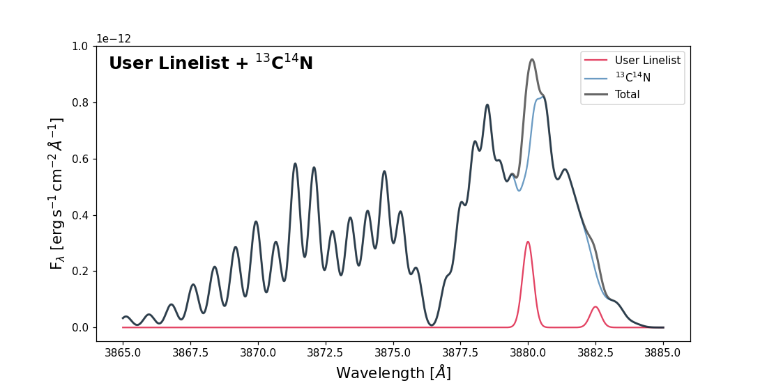
User-provided line list
Pass a custom line list as a pandas.DataFrame keyed by isotopologue
in linelists. The DataFrame must use the normalized column schema:
lambda_vac_A, A_ul, upper_id, lower_id, g_upper,
g_lower and if collisions are present you will also need:
lower_es_col, lower_v_col, lower_J_col, lower_sym_col, and E_lower_cm1_col.
Use from_user_linelist() to convert any custom-format table into this schema (see Utilities).
You can also mix user line lists with the built-in ones. You can name your isotopologues as you prefer, but for built-in line lists
we recommend keeping the default names. If you want to mix a user line list without collisions with a built-in one with collisions,
the user isotopologue name must follow the pattern <number><Capital Letter> to avoid errors. Here is an example:
from cometspec.modeling import from_user_linelist

# Your data in whatever column names you have
raw_ll = pd.DataFrame({
   "wave": [3880.0, 3882.5],   # Angstroms
   "A":    [1e6,    5e5],       # Einstein A [s^-1]
   "uid":  ["u1",   "u2"],      # upper state label
   "lid":  ["l1",   "l2"],      # lower state label
   "gu":   [3,      5],         # upper degeneracy
   "gl":   [1,      3],         # lower degeneracy
})

# Convert to the normalized schema
user_ll = from_user_linelist(
   raw_ll,
   lam_col="wave", A_col="A",
   upper_id_col="uid", lower_id_col="lid",
   g_upper_col="gu", g_lower_col="gl",
)

model_user = FluorescenceModel(
   pumping=irradiance,
   isotopologues=["1Fx", "13C14N"],
   window = (3865, 3885),
   linelists={"1Fx": user_ll},
   logN_by_iso={"1Fx": 12.5, "13C14N": 13.0},
   T=100.0,
   sigma=0.2,
   lsf_method="Gauss",
   include_rotations=True,
   A_min=1e4,
   f_col=-1,
)

plt.figure(figsize=(10, 5))
plt.text(0.02, 0.97, r"User Linelist + $^{13}$C$^{14}$N", transform=plt.gca().transAxes,
         fontsize=16, fontweight="bold", va="top")
plt.plot(model_user.model_by_iso["1Fx"][0], model_user.model_by_iso["1Fx"][1],
      c='crimson', alpha=0.8, label="User Linelist")
plt.plot(model_user.model_by_iso["13C14N"][0], model_user.model_by_iso["13C14N"][1],
      c='steelblue', alpha=0.8, label=r"$^{13}$C$^{14}$N")
plt.plot(model_user.model_wave, model_user.best_model, c='k', alpha=0.6, label="Total",
      lw=2)
plt.xlabel(r"Wavelength [$\AA$]", fontsize=14)
plt.ylabel(r"F$_\lambda$ [$\mathrm{erg}\,\mathrm{s}^{-1}\,\mathrm{cm}^{-2}\,\AA^{-1}$]",
      fontsize=14)
plt.legend()
plt.show()
If collisions are disabled, or if all isotopologues include collisions, you can name your own isotopologue as you prefer.
If your line list needs to include collisions, you will also need to provide the
lower_es_col, lower_v_col, lower_J_col, lower_sym_col, and E_lower_cm1_col columns.
Here is an example:
lines_wave = [3800, 3810, 3820, 3830, 3840]  # wavelengths in Angstroms
A = [1e4, 2e4, 3e4, 4e4, 5e4]  # Einstein A coefficients
upper_id_col = ['2', '3', '4', '5', '6']
lower_id_col = ['1', '2', '3', '4', '5']  # lower level IDs
g_upper_col = [1, 1, 1, 1, 1]  # statistical weights of the upper levels
g_lower_col = [2, 4, 6, 8, 10]  # statistical weights of the lower levels

loweres = ['X', 'X', 'X', 'X', 'X']  # electronic state
lowerv = [0, 0, 0, 0, 0]  # vibrational state
lowerJ = [0.5, 1.5, 2.5, 3.5, 4.5]  # J quantum numbers
lowersym = ['F1e', 'F1e', 'F1e', 'F1e', 'F1e']  # symmetry label
Elower = [1, 4, 9, 16, 25]  # energies with respect the ground state,cm^-1

custom_linelist_1 = pd.DataFrame({'WAVE': lines_wave,
                              'A_EINSTEIN': A,
                              'UPPER_ID': upper_id_col,
                              'LOWER_ID': lower_id_col,
                              'G_UPPER': g_upper_col,
                              'G_LOWER': g_lower_col,
                              'LOWER_ELECTRONIC_STATE': loweres,
                              'LOWER_VIBRATIONAL_STATE': lowerv,
                              'LOWER_J_LEVEL': lowerJ,
                              'LOWER_SYMMETRY': lowersym,
                              'E_LOWER': Elower
                              })

lines_custom = from_user_linelist(custom_linelist_1,
                              lam_col =  'WAVE',
                              A_col = 'A_EINSTEIN',
                              upper_id_col = 'UPPER_ID',
                              lower_id_col = 'LOWER_ID',
                              g_upper_col = 'G_UPPER',
                              g_lower_col = 'G_LOWER',
                              lower_es_col = 'LOWER_ELECTRONIC_STATE',
                              lower_v_col = 'LOWER_VIBRATIONAL_STATE',
                              lower_J_col = 'LOWER_J_LEVEL',
                              lower_sym_col = 'LOWER_SYMMETRY',
                              E_lower_cm1_col = 'E_LOWER',)

model_synth = FluorescenceModel(
            pumping=irradiance,
            window = (3865, 3885),
            isotopologues=['iso1'],
            window=(3700.0, 3890.0),
            linelists={'iso1': lines_custom},
            lsf=None,
            lsf_method="Gauss",
            sigma=0.5,
            A_min=1e3,
            logN_by_iso={'iso1': 12.0},
            f_col= 4,
            T=300.0,
            include_rotations=True
         )
Updating a model
update_model() lets you change any
parameter and re-synthesise. It must be called because the rate matrix and the level-population
solution have to be recalculated. There are two options: set the parameters directly on the model
instance, or pass them as keyword arguments to update_model. For example:
# Build once
model = FluorescenceModel(pumping=irradiance,
    isotopologues="12C14N", systems="BX",
    logN=14.0, T=100.0, sigma=0.2, lsf_method="Gauss",
)

model.sigma=0.01
model.T = 300

model.update_model(f_col=-1)
Key output values
After construction the model exposes several per-isotopologue diagnostics and parameters. Here are some examples:
model = FluorescenceModel(pumping=irradiance,
               isotopologues=["12C14N", "13C14N"],
               logN_by_iso={"12C14N": 14.0, "13C14N": 13.0},
               T=100.0, sigma=0.2, lsf_method="Gauss", f_col=-1)

dic = model.n_lines()
print("-"*20)
print("Source of line lists:")
di2 = model.print_linelist_origins()
print("-"*20)
# Photon and energy g-factors
print("Photon g-factor [s^-1]:", model.g_ph_by_iso)
print("Energy g-factor [erg s^-1]:", model.g_en_by_iso)
print("-"*20)
print('Sum of photon g-factors:', model.g_ph_sum_by_iso)
print("-"*20)

print('Sum of energy g-factors:', model.g_en_sum_by_iso)
print("-"*20)

df_lines = model.lines_by_iso['12C14N']
print(df_lines)

print('Model parameters:')
print('-----------------')
print('LogN by isotopologue:')
for param, value in model.logN_by_iso.items():
   print(f'  {param}: {value}')
print('f_col:', model.f_col)
print('T:', model.T)
print('sigma:', model.sigma)
print('lsf_method:', model.lsf_method)
Using config files
FluorescenceModelConfig is a plain dataclass that groups
all constructor parameters. It makes configurations easy to version, share,
and serialise.
from cometspec import FluorescenceModelConfig

cfg = FluorescenceModelConfig(
    isotopologues=["12C14N", "13C14N"],
    systems="BX",
    logN=14.0,
    logN_by_iso={"13C14N": 12.9},
    T=100.0,
    sigma=0.2,
    lsf_method="Gauss",
)

# Build a model from the config
model_from_cfg = FluorescenceModel(pumping=irradiance, config=cfg
)

# Configs are plain dataclasses — easy to serialise
import json, dataclasses
print(json.dumps(dataclasses.asdict(cfg), indent=2, default=str))
Any parameter in the config will override a keyword argument passed directly to the
FluorescenceModel constructor. For example, if the config has logN=14.0 and
you pass logN=13.0 to the constructor, the model will use logN=14.0 from the config.
Different line spread functions
Several LSFs are available. Pass the name of the one you want to the lsf_method parameter:
Gauss: a Gaussian line spread function.2Gauss: a double Gaussian line spread function.Lorentz: a Lorentzian line spread function.Gauss_Lorentz: Gaussian plus Lorentzian.
Each option requires its own set of keyword arguments:
Gauss:sigma2Gauss:sigma1,sigma2,ratio(Gaussian 1 over Gaussian 2)Lorentz:fwhm_LGauss_Lorentz:sigma_G,fwhm_L,ratio(Gaussian over Lorentzian)
You can also pass a custom LSF. In that case the lsf parameter must be a callable
that takes a wavelength array as input and returns the LSF kernel.
References
The remaining references for the other line lists can be found at load_default_transitions().