MCMC Fitting

fit_mcmc() runs an emcee ensemble sampler on a FluorescenceModel. Priors are uniform; the priors dictionary controls both which parameters are free and their allowed ranges. Parameters absent from priors are fixed at their current values.

All examples use synthetic spectra generated from a known model with Gaussian noise added — no observational data is required.

We recommend checking the fit_mcmc() method for the full list of available parameters and options.

Sections

• Single-isotopologue fit

• Multi-isotopologue fit

• LSF fitting

• Plotting results

• Extracting results

• Parallel MCMC

• Using config files

• Save and Load MCMC results

---

Single-isotopologue fit

Pass the observed DataFrame and wavelength window when constructing the model, then call fit_mcmc() with the desired prior ranges. When creating the Fluorescence model you have the option to specify the columns in your DataFrame that contain the wavelength, flux, error, and continuum data; you can change them using the wave_col, flux_col, error_col, and continuum_col parameters.

from cometspec.helper import open_kurucz_irradiance, open_hall_anderson_irradiance
from cometspec import FluorescenceModel
from matplotlib import pyplot as plt
import numpy as np
import pandas as pd

irradiance = open_kurucz_irradiance()

model = FluorescenceModel(
    window=(3870, 3885),
    pumping=irradiance,
    isotopologues="12C14N",
    systems=['BX', 'AX_dv1'],
    sigma=0.05,
    logQ=-1,
    logN=14.0,
    T=200,
    v_kms=0,
    lsf_method="Gauss",
    wave_col="WAVE",
    flux_col="FLUX",
    error_col="ERR",
    continuum_col="CONTINUUM",
)

# add noise
data_flux = model.best_model + np.random.normal(0, np.max(model.best_model)*0.05,
                                                    size=model.model_wave.shape)
data = pd.DataFrame({'WAVE': model.model_wave,
                    'FLUX': data_flux,
                    'ERR':np.max(model.best_model)*0.05,
                    'CONTINUUM': np.zeros_like(model.model_wave)})

results = model.fit_mcmc(
                data=data,
                nwalkers=10,
                nsteps=500,
                priors={
                    "logN":  (12.0, 16.0),
                    "T":     (50.0, 300.0),
                    "v_kms": (-2.0, 2.0),
                },
                    make_plots=False,
                )

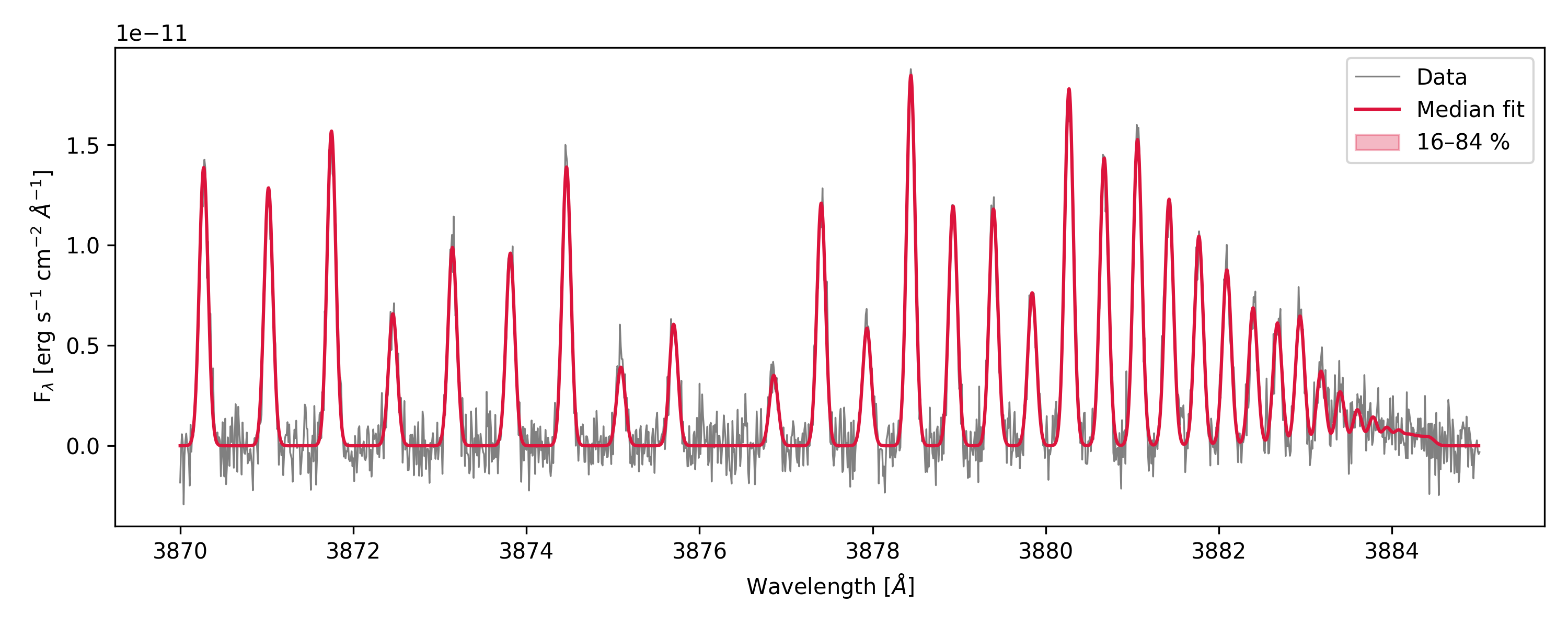
print("Median logN :", model.median_params["logN"])
print("Median T    :", model.median_params["T"])

plt.figure(figsize=(10, 4))
plt.plot(data["WAVE"], data["FLUX"],
        color="gray", lw=0.8, label="Data")
plt.plot(model.model_wave, model.median_model,
        color="crimson", lw=1.5, label="Median fit")
plt.fill_between(
    model.model_wave,
    model.model_p16, model.model_p84,
    alpha=0.3, color="crimson", label="16–84 %",
)
plt.xlabel(r"Wavelength [$\AA$]")
plt.ylabel(r"F$_\lambda$ [erg s$^{-1}$ cm$^{-2}$ $\AA^{-1}$]")
plt.legend()
plt.tight_layout()
plt.show()

The main attributes of FluorescenceModel available after fitting are the updated model parameters and the following:

• param_keys (names of the fitted parameters)

• median_params (median values of the fitted parameters)

• up_errors_params (upper errors of the fitted parameters, from the 84th percentile to the median)

• low_errors_params (lower errors of the fitted parameters, from the median to the 16th percentile)

• samples_pruned (the MCMC sample chain after burn-in and pruning, if applicable)

• lnprob_pruned (log-probability values corresponding to the pruned sample chain)

• median_model (median model spectrum)

• best_model (best-fit model spectrum, same as the median model)

• model_wave (updated model wavelength grid)

• model_p16 (16th percentile model spectrum)

• model_p84 (84th percentile model spectrum)

• model_by_iso (model spectra split by isotopologue, if multiple isotopologues are present)

---

Multi-isotopologue fit

Use isotopologue-specific prior keys — logN_13C14N, T_13C14N, etc. — to give each species its own parameter range. Any iso-specific key not found falls back to the shared key (logN_by_iso, T_by_iso, …), and if that is also not found, it falls back to the default value (logN, T, …). We highly encourage setting all isotopologues in the by_iso parameters (if used) when building the model, in order to avoid confusion.

model2 = FluorescenceModel(
    window=(3870, 3885),
    pumping=irradiance,
    isotopologues=["12C14N", "13C14N"],
    systems=['BX', 'AX_dv1'],
    sigma=0.05,
    logQ_by_iso={"12C14N": -1, "13C14N": -2},
    logN_by_iso={"12C14N": 14.0, "13C14N": 13.5},
    T=200,
    v_kms=0,
    lsf_method="Gauss",
    wave_col="WAVE",
    flux_col="FLUX",
    error_col="ERR",
    continuum_col="CONTINUUM",
)

# add noise
data_flux = model2.best_model + np.random.normal(0, np.max(model2.best_model)*0.05,
                                                    size=model2.model_wave.shape)
data = pd.DataFrame({'WAVE': model2.model_wave,
                    'FLUX': data_flux,
                    'ERR':np.max(model2.best_model)*0.05,
                    'CONTINUUM': np.zeros_like(model2.model_wave)})


results2 = model2.fit_mcmc(
    data=data,
nwalkers=20,
nsteps=100,
priors={
    "logN_12C14N": (12.0, 16.0),
    "logN_13C14N": (11.0, 15.0),
    "T":           (50.0, 300.0),
},
make_plots=False,
n_cores=2
)



plt.figure(figsize=(10, 4))
plt.plot(data["WAVE"], data["FLUX"],
        color="gray", lw=0.8, label="Data")
plt.plot(model2.model_wave, model2.median_model,
        color="crimson", lw=1.5, label="Median fit")
for iso in model2.isotopologues:
    plt.plot(model2.model_by_iso[iso][0], model2.model_by_iso[iso][1],
            lw=1.0, label=f"Median fit {iso}")
plt.fill_between(
    model2.model_wave,
    model2.model_p16, model2.model_p84,
    alpha=0.3, color="crimson", label="16–84 %",
)
plt.xlabel(r"Wavelength [$\AA$]")
plt.ylabel(r"F$_\lambda$ [erg s$^{-1}$ cm$^{-2}$ $\AA^{-1}$]")
plt.legend()
plt.tight_layout()
plt.show()

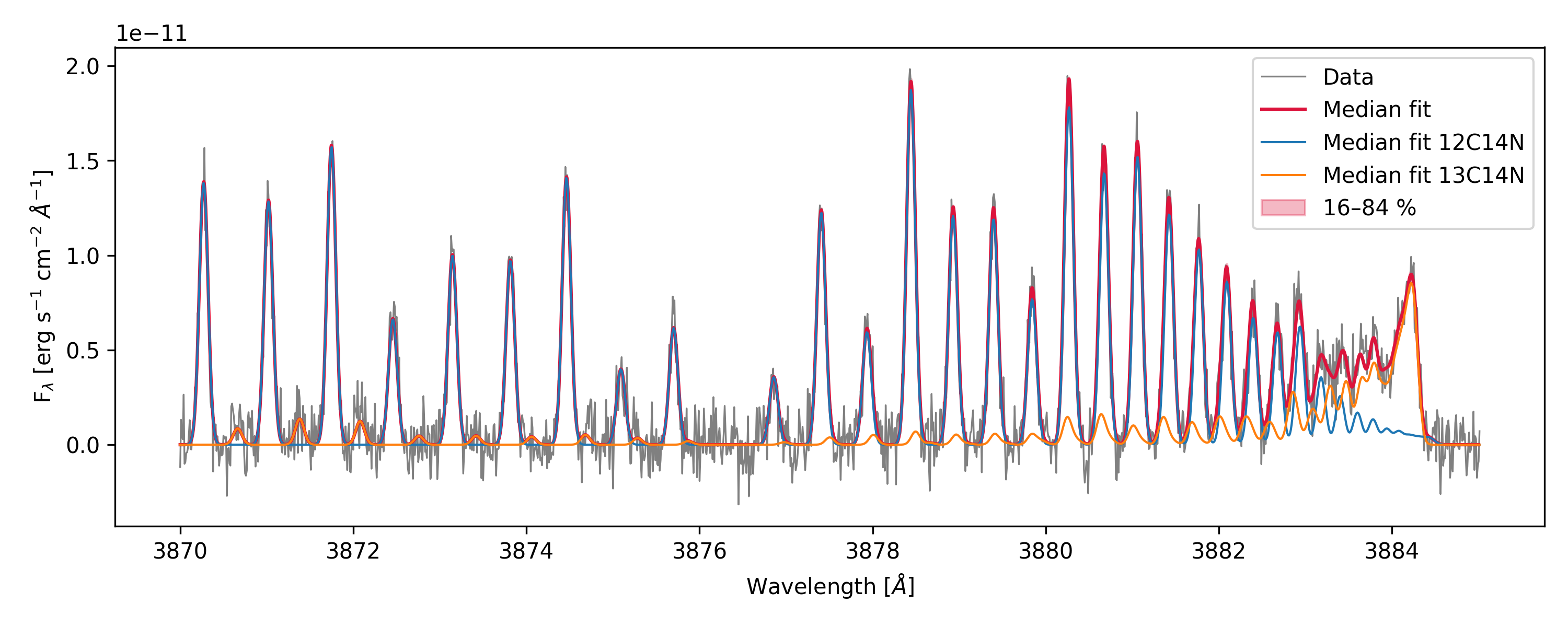
In this example T is shared between both isotopologues, while logN has separate priors and fitted values. logQ_by_iso is not present in the priors, so it is fixed at the values given in the model constructor.

---

LSF fitting

You can also include in the priors any of the LSF parameters (sigma, sigma1, sigma2, sigma_G, fwhm_L, ratio) to fit the line spread function together with the physical parameters (while being consistent with the lsf_method).

print('Original sigma:', model.sigma)

model.fit_mcmc(
    nwalkers=10, nsteps=100,
    priors={'logN': (12.0, 16.0), 'sigma': (0.01, 0.1)},
    make_plots=False,
)

print('Fitted sigma:', model.median_params.get('sigma'))
print('Fitted sigma:', model.sigma)

The full list of fittable parameters is: logN, logQ, T, v_kms, dlam, their per-isotopologue variants (e.g. logN_13C14N), and LSF parameters sigma, sigma1, sigma2, sigma_G, fwhm_L, ratio depending on the chosen lsf_method. Additionally, if you provide the LSF via a custom callable, it will be used for the fit, so you can ignore the LSF priors.

def lsf(x):
    """Example of a custom LSF function: a simple Gaussian."""
    import numpy as np  # imported inside so multiprocessing workers have access
    sigma = 0.02  # Standard deviation of the Gaussian
    return (1 / (sigma * np.sqrt(2 * np.pi))) * np.exp(-0.5 * ((x) / sigma) ** 2)

model = FluorescenceModel(pumping=irradiance,
                        isotopologues=['12C14N'],
                        systems=['B-X'],
                        lsf=lsf,
                        A_min=1e3,
                        logN = 14,
                        logQ= -1,
                        T=300.0,
                        window=(3865.0, 3885.0),
                        wave_col="WAVE",
                        flux_col="FLUX",
                        error_col="ERR",
                        continuum_col="CONTINUUM",
                        a=7)
# add noise
data_flux = model.best_model + np.random.normal(0, np.max(model.best_model)*0.05,
                                                size=model.model_wave.shape)
data = pd.DataFrame({'WAVE': model.model_wave, 'FLUX': data_flux,
                    'ERR':np.max(model.best_model)*0.05,
                    'CONTINUUM': np.zeros_like(model.model_wave)})

model.fit_mcmc(
    data=data,
    nwalkers=20, nsteps=300,
    priors={'logN': (12.0, 16.0)},
    make_plots=False,
    lsf=model.lsf # This needs to be set if it is a custom LSF
)

---

Plotting results

fit_mcmc() saves and shows diagnostic figures when make_plots=True (the default). With fig_file you can specify a custom path prefix for the corner and fit plots.

priors = {
    'logN': (5, 20),
    'logQ': (-4, 1),
    'T': (10, 400),
}

model = FluorescenceModel(
    window = (3866.0, 3884.0),
    pumping=irradiance,
    lsf_method="Gauss",
    A_min=1e4,
    name=f'CN_Model',
    sigma = 0.01,
    logN=12.0,
    v_kms=0.0,
    T=300.0,
    logQ=-1.0,
    isotopologues=['12C14N'],
    wave_col="WAVE",
    flux_col="FLUX",
    error_col="ERR",
    continuum_col="CONTINUUM",
)

# add noise
data_flux = model.best_model + np.random.normal(0, np.max(model.best_model)*0.05,
                                                size=model.model_wave.shape)
data = pd.DataFrame({'WAVE': model.model_wave, 'FLUX': data_flux,
                    'ERR':np.max(model.best_model)*0.05,
                    'CONTINUUM': np.zeros_like(model.model_wave)})

model.fit_mcmc(data = data,
        nwalkers=10,
        nsteps=2000,
        priors=priors,
        make_plots=True,
        progress=True,
        A_min=1e5,
        a=3,
        fig_file='example',
        )

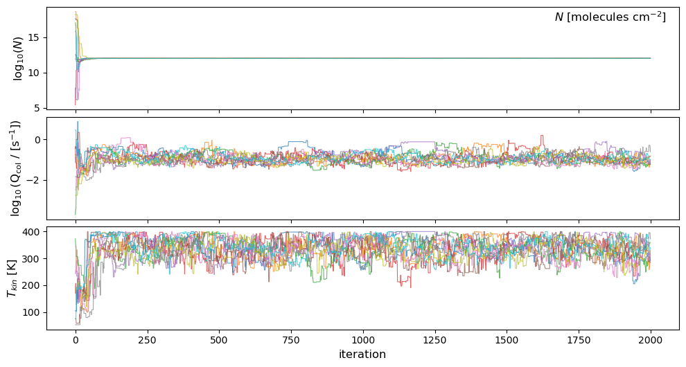
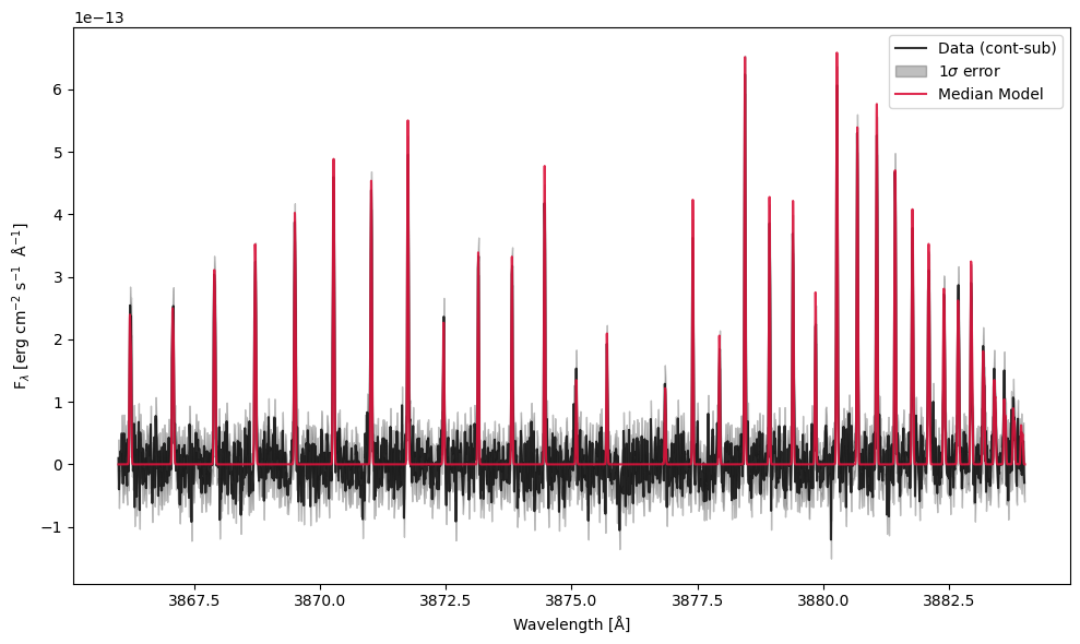
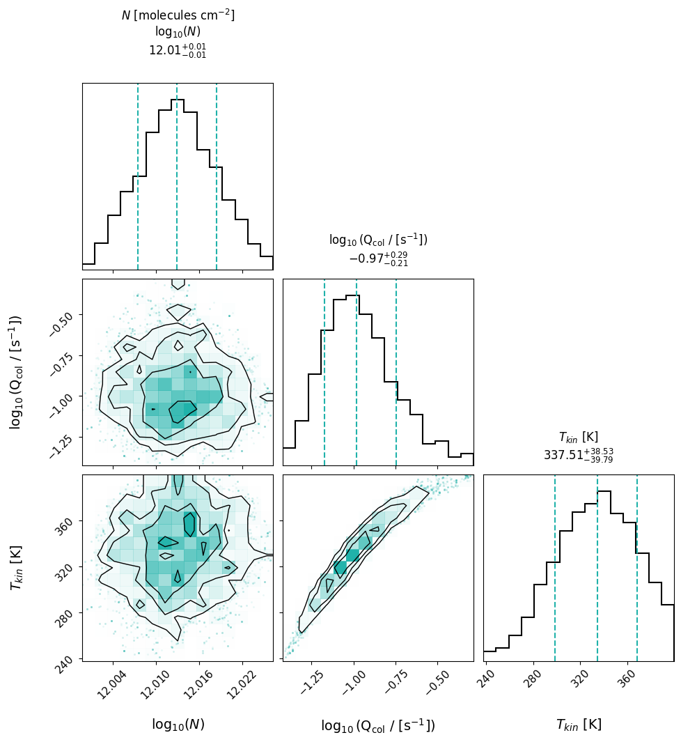
This code will produce a traces plot where you can see the trace of each walker throughout the MCMC steps for each fitted parameter, a corner plot showing the posterior distributions and covariances of the fitted parameters, and a fit plot showing the observed spectrum with its error and the median model fit. All three are saved as pdf files.

If you want to recreate the fit, you can use any of the attributes above to access the model. The traces cannot be regenerated, as all the walkers were collapsed and pruned. If you want to recreate the corner plot, you can do so using samples_pruned. Here is an example using the corner package:

param_labels = model.param_keys
import corner
fig = corner.corner(
            model.samples_pruned,
            labels=param_labels,
            title_kwargs={'fontsize': 12, 'y': 1.05},
            title_fmt=".2f",
            use_math_text=True,
            bins=15,
            quantiles=[0.16, 0.5, 0.84],
            show_titles=True,
            color='crimson',
            hist_kwargs={'color': 'black', 'linewidth': 1.5},
            contour_kwargs={'linewidths': 1, 'colors': 'black'},
            label_kwargs={'fontsize': 11},
            fig=plt.figure(figsize=(8, 8)),
        )
axes = np.array(fig.axes).reshape((len(param_labels), len(param_labels)))

for i in range(len(param_labels)):
    ax = axes[i, i]
    q16, q50, q84 = np.quantile(model.samples_pruned[:, i], [0.16, 0.5, 0.84])
    q_minus, q_plus = q50 - q16, q84 - q50
    title = (
        f"{param_labels[i]}\n"
        rf"=${q50:.2f}_{{-{q_minus:.2f}}}^{{+{q_plus:.2f}}}$"
    )
    ax.set_title(title, fontsize=12, y=1.05)
plt.show()

And then you can edit it as you prefer.

---

Extracting results

All posterior summaries are stored as instance attributes of FluorescenceModel after the fit. As mentioned before:

• param_keys (names of the fitted parameters)

• median_params (median values of the fitted parameters)

• up_errors_params (upper errors of the fitted parameters, from the 84th percentile to the median)

• low_errors_params (lower errors of the fitted parameters, from the median to the 16th percentile)

• samples_pruned (the MCMC sample chain after burn-in and pruning, if applicable)

• lnprob_pruned (log-probability values corresponding to the pruned sample chain)

• median_model (median model spectrum)

• best_model (best-fit model spectrum, same as the median model)

• model_wave (updated model wavelength grid)

• model_p16 (16th percentile model spectrum)

• model_p84 (84th percentile model spectrum)

• model_by_iso (model spectra split by isotopologue, if multiple isotopologues are present)

print("Fitted parameters:", model.param_keys)
print("Medians          :", model.median_params)
print("Upper errors (1σ):", model.up_errors_params)
print("Lower errors (1σ):", model.low_errors_params)

# Formatted column density with asymmetric errors
logN_med = model.median_params["logN"]
logN_up  = model.up_errors_params["logN"]
logN_lo  = model.low_errors_params["logN"]
print(f"log N = {logN_med:.2f} +{logN_up:.2f} / -{logN_lo:.2f}  [cm^-2]")

# Full pruned sample chain (shape: n_samples × n_params)
print("Sample chain shape:", model.samples_pruned.shape)

---

Parallel MCMC

The walker likelihood evaluations are independent within each emcee step, so they can be parallelized across CPU cores. CometSpec uses the multiprocess package. It is installed automatically as a CometSpec dependency. Pass n_cores>1 either when constructing the model (stored as self.n_cores) or directly to fit_mcmc().

results_par = model.fit_mcmc(
    nwalkers=20,
    nsteps=500,
    n_cores=8,                # parallelize walkers across 8 cores
    priors={
        "logN":  (12.0, 16.0),
        "T":     (50.0, 300.0),
        "v_kms": (-2.0, 2.0),
    },
    make_plots=False,
)

Important

Running from a ``.py`` script: when n_cores > 1, the call to fit_mcmc() (or cometspec.mcmc.mcmc_fitting()) must be guarded by if __name__ == "__main__":. Each spawn worker re-imports the user script, and without the guard the parallel call would re-execute on import and Python aborts with a clear RuntimeError.

# my_script.py
import cometspec

def run_fit():
    model = cometspec.FluorescenceModel(...)
    return model.fit_mcmc(n_cores=8, ...)

if __name__ == "__main__":
    results = run_fit()

Imports, function definitions, and helper code stay at module level — only the actual fit_mcmc invocation needs to be inside the guard. The guard is not needed in Jupyter notebooks, nor when n_cores is None or 1.

Note

When using n_cores > 1, any module a custom lsf relies on (numpy, scipy, …) must be imported inside the function so the worker processes can recognize it. Example:

def lsf(x):
    import numpy as np
    sigma = 0.02
    return (1 / (sigma * np.sqrt(2 * np.pi))) * np.exp(-0.5 * (x / sigma) ** 2)

---

Using config files

MCMCFitConfig groups all MCMC options into a single dataclass, mirroring FluorescenceModelConfig for model setup. Again, the default is that any parameter present in the config file will overwrite any kwarg passed to the function.

from cometspec import MCMCFitConfig

mcmc_cfg = MCMCFitConfig(
    nwalkers=10,
    nsteps=100,
    n_cores=2,
    make_plots=False,
    priors={
        "logN":  (12.0, 16.0),
        "T":     (50.0, 300.0),
        "v_kms": (-2.0, 2.0),
    },
)

results_cfg = model.fit_mcmc(config=mcmc_cfg)

---

Save and Load MCMC results

In order to save and then access your MCMC results in the future, you can use the methods save() and load() respectively, which save and load a pickle of the model.

model.save(filename=f'result.pkl')

model = FluorescenceModel.load(filename=f'result.pkl')