Utilities
The cometspec.helper module provides standalone utilities for
solar irradiance, seeing corrections, and line list handling.
Sections
Solar irradiance
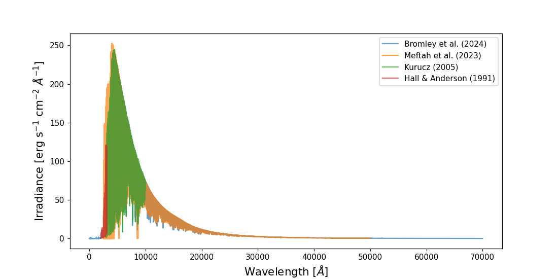
CometSpec comes with four different solar irradiance references by default: Kurucz (2005) [1], covering 2990 to 10,000 Å; Hall & Anderson (1991) [2], for the UV range of 2000 to 2990 Å (it can be extended up to 3100.9 Å, but the default is 2990 to avoid overlap with Kurucz); Meftah et al. (2023) [3], covering the range of 2500 to 50,000 Å; and Bromley et al. (2024) [4], covering from 1 to 70,000 Å.
The wavelength range used to filter the default transition linelists is taken directly from the
minimum and maximum wavelengths of the solar irradiance (pumping) spectrum supplied to the model.
To extend or restrict that range, build or concatenate a pumping spectrum that covers the desired
range and pass it as pumping to FluorescenceModel.
If you concatenate different solar irradiance references, it is recommended that (i) the spectra do not overlap and (ii) their continua match,
as there are differences among them.
Default functions:
from cometspec.helper import open_kurucz_irradiance
from cometspec.helper import open_hall_anderson_irradiance
from cometspec.helper import open_meftah_irradiance
from cometspec.helper import open_bromley_irradiance
import numpy as np
import pandas as pd
import matplotlib.pyplot as plt


irradiance_kurucz = open_kurucz_irradiance()
irradiance_hall_anderson = open_hall_anderson_irradiance(wave_max_AA=10000)
                                 # just a large wavelength to cover the max.
irradiance_meftah = open_meftah_irradiance()
irradiance_bromley = open_bromley_irradiance()

plt.figure(figsize=(10, 5))
plt.plot(irradiance_bromley['WAVE'], irradiance_bromley['FLUX'],
         label='Bromley et al. (2024)', alpha=0.7)
plt.plot(irradiance_meftah['WAVE'], irradiance_meftah['FLUX'],
         label='Meftah et al. (2023)', alpha=0.7)
plt.plot(irradiance_kurucz['WAVE'], irradiance_kurucz['FLUX'],
         label='Kurucz (2005)', alpha=0.7)
plt.plot(irradiance_hall_anderson['WAVE'], irradiance_hall_anderson['FLUX'],
         label='Hall & Anderson (1991)', alpha=0.7)
plt.xlabel(r"Wavelength [$\AA$]", fontsize=14)
plt.ylabel(r"Irradiance [erg s$^{-1}$ cm$^{-2}$ $\AA^{-1}$]", fontsize=14)
plt.legend()
plt.show()
All functions return pandas.DataFrame objects and can be passed directly to
the pumping argument of FluorescenceModel. The only requirement for a
user-provided one is that it must be a DataFrame with columns named WAVE and FLUX.
Slit-loss error on production rates
Within the FluorescenceModel, you can call
add_slit_loss_error() to add the estimated slit-loss error to the model’s error.
This method is a wrapper around add_slit_loss_error_scalar(), which computes the slit-loss error for a
given set of parameters. You can call this function directly if you want to compute the slit-loss for any value (in log space) that is
proportional to the flux, e.g. apply the function to \(\log_{10}(\mathbf{Flux})\) or \(\log_{10}(N)\), where \(N\) is the column density.
Here is an example of how to use it:
from cometspec.helper import add_slit_loss_error_scalar

logQ_err_nominal = 0.05   # initial uncertainty on log space

logQ_err_total = add_slit_loss_error_scalar(
    logQ_err_nominal,
    lambda_nm=388.3, # wavelength in which the slit-loss is calculated
    aperture={"type": "circular", "radius_arcsec": .5},
    eps_min_arcsec_500=0.7, # minimum seeing at 500 nm in arcseconds
    eps_max_arcsec_500=1.2, # maximum seeing at 500 nm in arcseconds
    zmin_deg=30.0, # minimum zenith angle in degrees
    zmax_deg=60.0, # maximum zenith angle in degrees
)

print(f"logQ error (MCMC only): {logQ_err_nominal:.3f}")
print(f"logQ error (total)    : {logQ_err_total:.3f}")
Line list utilities
Regarding the line list to use, there are two useful functions: one to convert a given table into the
internal format that cometspec uses, and another to load the default line lists that are packaged with cometspec.
The latter can be useful, for instance, if you want to apply additional filters or to inspect which lines are available.
The current table format does not contain all the upper-level information of a transition, so for more complex filtering we recommend providing
your own line list. However, in the Jupyter notebook available on the
GitHub repo (link) there are more examples of this filtering and of how
the line lists were created. For further details on the default line lists, we refer to our publication [5].
Converting a custom line list
from_user_linelist() maps your column names to the
normalized internal schema (lambda_vac_A, A_ul, upper_id,
lower_id, g_upper, g_lower, and if collisions are to be included you will need
lower_es_col, lower_v_col, lower_J_col, lower_sym_col and E_lower_cm1_col), check the
API documentation for more details.
import pandas as pd
from cometspec.modeling import from_user_linelist

raw = pd.DataFrame({
    "wave": [3883.0, 3884.5],
    "A":    [1e6,    5e5],
    "uid":  ["u1",   "u2"],
    "lid":  ["l1",   "l2"],
    "gu":   [3,      5],
    "gl":   [1,      3],
})

normalized = from_user_linelist(
    raw,
    lam_col="wave", A_col="A",
    upper_id_col="uid", lower_id_col="lid",
    g_upper_col="gu", g_lower_col="gl",
)
print(normalized)
Loading built-in line lists as DataFrames
load_default_transitions() loads the packaged line
list for any supported species and returns it as a dict of DataFrames, one
per isotopologue.
from cometspec.modeling import load_default_transitions

# Load CN B-X for 12C14N and C2 Swan for 12C2
lls = load_default_transitions(
    isotopologues=["12C14N", "12C2"],
)
print(lls["12C14N"].head())
print(f"12C14N lines: {len(lls['12C14N'])}")

print(lls["12C2"].head())
print(f"12C2 lines: {len(lls['12C2'])}")
Check the API documentation for more details on additional parameters of the functions (e.g. the default minimum Einstein coefficient \(A_{ul}\)).